Transition Matrix Method
for Polymers Confined to a Lattice, Part 1

Polymers can assume a huge number of states (conformations) which makes the calculation of their thermodynamical properties extremely difficult. To simplify the problem, the number of available states has to be reduced, which is often done by assuming discrete states. One of the most popular models is the quasi-crystalline lattice model where groups of atoms are treated as single interaction units which are restricted to a lattice.^1,2 As has been shown by many authors, lattice problems may be best solved using a transition matrix formalism.^3-8
The matrix method is very convenient and can be adapted to solve many lattice walk problems. One of the oldest models that utilizes this formalism was developed by DiMarzio and Rubin (1971) to describe the behavior of polymer lattice chains in confined space.^3-5 

     2D Lattice Polymer Chain

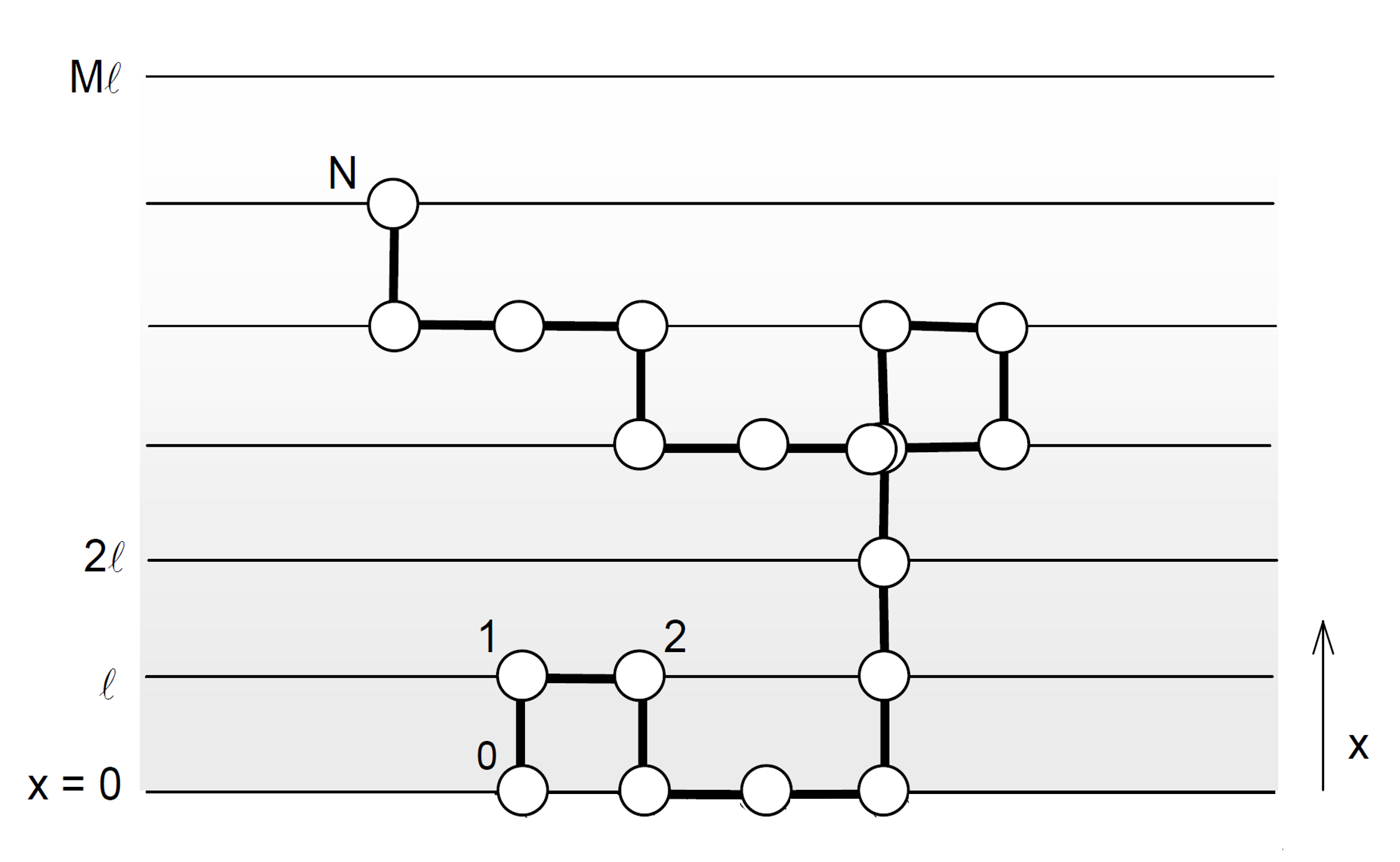
Let us consider a lattice chain near an impermeable interface. The lattice can be considered as an array of layers numbered i = 1, 2, ..., M with sites similar to the surface layer (see figure above). The interface corresponds to the y - z lattice plane through the point x = 0. Successive lattice planes through x = l, 2l, 3l.. represent the solution phase where l is the lattice constant. Each site is surrounded by z nearest-neighbor sites. λ₀ z sites are located in the same layer and λ₁ z = z (1 - λ₀) / 2 in one of the adjacent layers. Far from the surface plane, all random walk configurations of a given length are equally likely. However walks of the same length that touch the interface will have different probabilities, depending on the interaction energy ε_pw between the chain segments and the interface.

Consider a chain of N + 1 repeat units that has its first unit in the surface layer, i = 0. This situation is equivalent to a N-step restricted random walk that starts in the surface layer. Obviously, after N steps, the random walker can be located in any one of the layers from x = 0 to x = N. Therefore, at the Nth step N + 1 probabilities have to be considered: G(N, 0), G(N, 1l)...G(N, Nl), where G(N, kl) is the unnormalized probability that a walk ends in the kth lattice layer at the Nth step. If the last segment is in layer k ≥ 1, then the last but one has to be in layer k - 1, k or k + 1. The recurrence relation for this problem is evidently

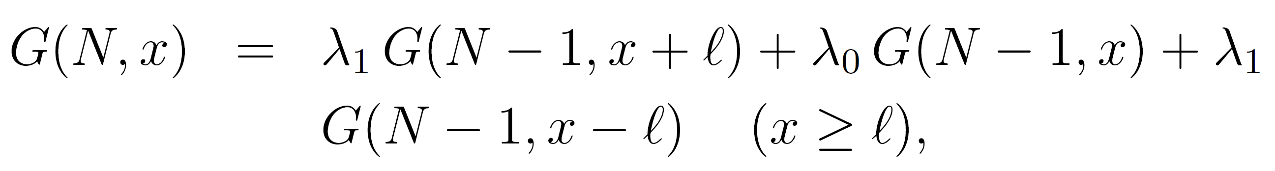
and for the segments at the interface:

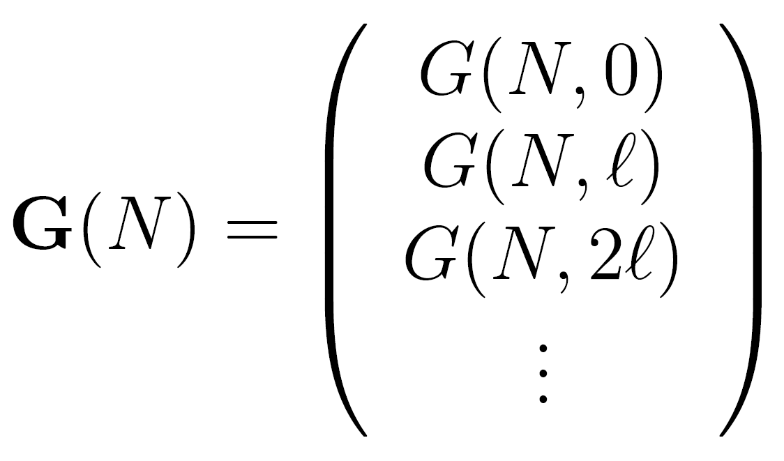
where χ_s = ε_pw / kT is a dimensionless adsorption energy parameter first introduced by Silberberg.¹⁰ The N + 1 recurrence relations can be written in matrix form as

where G(N) is the column vector of all end segment probabilities G(N,i):

The transition probability matrix W is given by

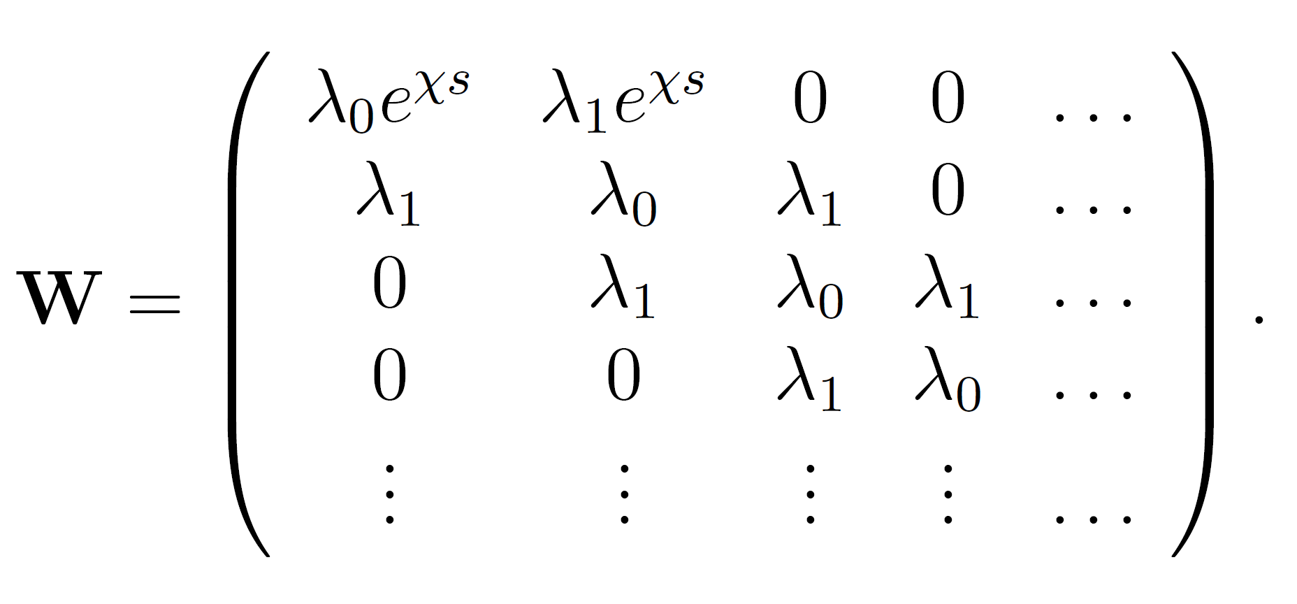
As the starting vector we choose G(0) = (e^χ_s, 0, 0,...,0). This choice for G(0) assures that all random walks start in the surface layer. This can be easily verified. For example, two iterations result in

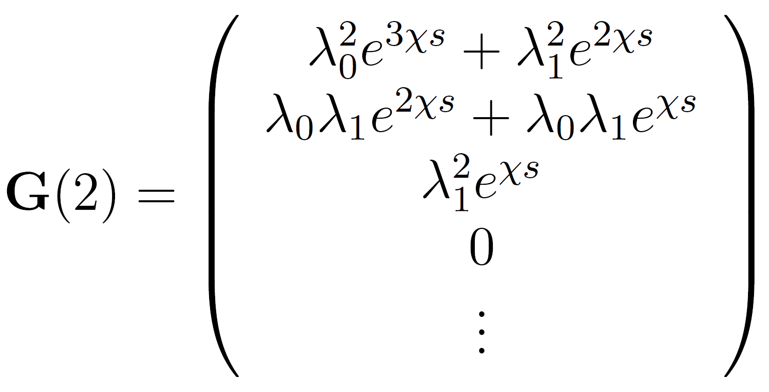
In this matrix, each polymer conformation is weighted by the proper Boltzmann factor. For example, for three segments (two bonds) with the first and last unit in the surface layer, the unnormalized probability reads

The first term is the probability that all three units (connected by 2 bonds) lie in the surface layer, whereas the second term is the probability that only the first and third unit touch the surface.
As will be shown in part 2, the conformational partition function Q_N+1 along with various statistical properties can be directly calculated from the relative probabilities G(0)....G(N). The matrix procedure outlined above, however, is only applicable to lattice polymers in the melt or theta state where the effects of monomer-solvent interaction and excluded volume can be neglected. For all other cases, the matrix has to be modified to incorporate both effects in each layer. This leads to complicated expressions which have to be solved by an iterative procedure.^6,7

References & Notes

1. P. J. Flory, J. Chem. Phys. 9, 660 (1941); 10, 51 (1942)
2. M. L. Huggins, J. Phys. Chem. 46, 151 (1942); J. Am. Chem. Soc. 64, 1712 (1942)
3. E. A. DiMarzio,, J. Chem. Phys., 42, 2101 (1965)
4. R. J. Rubin, J. Chem. Phys., 43, 2392 (1965)
5. E. A. DiMarzio & R. J. Rubin, J. Chem. Phys., 55, 4318 (1971)
6. R. J. Roe, J. Chem. Phys., 60, 4192 (1974)
7. J. M. H. M. Scheutjens & G. J. Fleer, J. Phys. Chem. 83, 1620 (1979) & 84, 178 (1980)

8. The transition matrix formalism has also been used by Flory to calculate the conformations
   of linear polymer chains using discrete rotational isomeric states.⁹

9. P. J. Flory, Statistical Mechanics of Chain Molecules, Wiley, New York (1969)
10. A. Silberberg, J. Chem. Phys., 46, 1105 (1967)